Decision Trees in Classification
The Gist of Decision Trees
Decision trees aren’t the most accurate method of classification, as they often lead to overfitting, but it’s still a very intuitive way of understanding how classification works.
A decision tree is basically a collection of decision nodes, where if-thens rule. Each tier of nodes is basically a step down from significance of information, or in other words, the first node will likely contain the most useful information for the model, while the second tier of nodes will contain the second most useful information, and so forth.
Splits in nodes have to be discrete; you either have high assets or low assets, you have high savings, low savings, or medium savings, your income is above \$50K, or less than or equal to \$50K. Depending on the algorithm used, you might have binary choices between each node, or you can have more. And the algorithms will try to optimize for different heuristics. So if we were to pretend that income weren’t a categorical variable, and it were continuous, one algorithm might find an optimal splitting point between 20 and 30K, while another one might find it to be at 35K. One might break it down into two decisions, and another might break it down into three. So if it starts out continuous, it will be discretized.
Leaf-nodes may have different target values contained within them, there usually aren’t pure leaf-nodes, where the node represents one value. Explicitly, a terminating node might contain 3⁄5 people that are classified as bad credit-risk, and 2⁄5 people that are classified as good credit risk. So a decision tree might report that a classification in credit-risk for some customer is bad, with 60% confidence, as determined by the 3⁄5 of customers in this node having bad credit risk.
Requirements
- Decision trees represent supervised learning, so they require preclassified target variables. A training set must be provided, with the values of the target variable.
- The training set should be deep and diverse, as the algorithm should have many combinations of the types of records for any possible classifications (so that some edge-case doesn’t slip through and get mis-classified). Decision trees learn by example and need strong examples.
- Target attribute classes must be discrete; if they are continuous, they must be discretized in advance.
Algorithms
In the code toward the bottom of the notebook, you will notice that the tree is instantiated with the argument critereon='gini'. This specifies which algorithm will be used to construct the tree. DecisionTreeClassifier() has two criteria that are supported: ‘gini’ for Gini impurity and ‘entropy’ for information gain. Gini impurity is the default. Both will yield around the same results but due to entropy requiring logarithmic calculations, it’s more computationally expensive. There are many algorithms that can build a decision tree, like CART (Classification and Regression Tree) and C4.5.
import pandas as pd
import numpy as np
from sklearn import tree, preprocessing
from sklearn.preprocessing import LabelEncoder
from IPython.display import display, Image

pd.set_option('display.notebook_repr_html', True)
df = pd.read_csv('Clem3Training.txt')display(df.head())| age | workclass | demogweight | education | education-num | marital-status | occupation | relationship | race | sex | capital-gain | capital-loss | hours-per-week | native-country | income | |
|---|---|---|---|---|---|---|---|---|---|---|---|---|---|---|---|
| 0 | 39 | State-gov | 77516 | Bachelors | 13 | Never-married | Adm-clerical | Not-in-family | White | Male | 2174 | 0 | 40 | United-States | <=50K. |
| 1 | 50 | Self-emp-not-inc | 83311 | Bachelors | 13 | Married-civ-spouse | Exec-managerial | Husband | White | Male | 0 | 0 | 13 | United-States | <=50K. |
| 2 | 38 | Private | 215646 | HS-grad | 9 | Divorced | Handlers-cleaners | Not-in-family | White | Male | 0 | 0 | 40 | United-States | <=50K. |
| 3 | 53 | Private | 234721 | 11th | 7 | Married-civ-spouse | Handlers-cleaners | Husband | Black | Male | 0 | 0 | 40 | United-States | <=50K. |
| 4 | 28 | Private | 338409 | Bachelors | 13 | Married-civ-spouse | Prof-specialty | Wife | Black | Female | 0 | 0 | 40 | Cuba | <=50K. |
Data Preprocessing
Categorization
Some of these predictor variables have needless complexity. I mean, maybe being divorced you’re going to be more susceptible to behave in a different way with money, or maybe people that are divorced tend to behave a certain way with money, but it isn’t that likely, so we’ll just break all of these specific marital statuses down into two, ‘y’ for yes, married, and ‘n’ for no, not married. The same will be done for workclass, as private companies function very differently than governmental companies.
#I'm adding a new column w/ same values b/c I don't want to overwrite original data
df['marital-status-cats'] = df['marital-status'].copy()
df['workclass-cats'] = df['workclass'].copy()
#So that I know which values to feed into the renaming dictionary
print(df['workclass'].unique())
print(df['marital-status-cats'].unique())
#This dictionary is interpreted as; in column of df, the key will be replaced by the value
category_replacement = {'marital-status-cats' : {'Married-civ-spouse': 'y', 'Married-AF-spouse': 'y', 'Married-spouse-absent': 'y',
'Divorced': 'n', 'Widowed': 'n', 'Separated': 'n', 'Never-married': 'n'},
'workclass-cats': {'Federal-gov': 'Gov', 'Local-gov': 'Gov', 'State-gov': 'Gov', 'Self-emp-inc': 'Self',
'Self-emp-not-inc': 'Self'}}['State-gov' 'Self-emp-not-inc' 'Private' 'Federal-gov' 'Local-gov' '?'
'Self-emp-inc' 'Without-pay' 'Never-worked']
['Never-married' 'Married-civ-spouse' 'Divorced' 'Married-spouse-absent'
'Separated' 'Married-AF-spouse' 'Widowed']df.replace(category_replacement, inplace=True)df['marital-status-cats'] = pd.Categorical(df['marital-status-cats'])
df['marital-status-cats'].cat.categories
df['workclass-cats'] = pd.Categorical(df['workclass-cats'])
df['workclass-cats'].cat.categories
display(df.head())| age | workclass | demogweight | education | education-num | marital-status | occupation | relationship | race | sex | capital-gain | capital-loss | hours-per-week | native-country | income | marital-status-cats | workclass-cats | |
|---|---|---|---|---|---|---|---|---|---|---|---|---|---|---|---|---|---|
| 0 | 39 | State-gov | 77516 | Bachelors | 13 | Never-married | Adm-clerical | Not-in-family | White | Male | 2174 | 0 | 40 | United-States | <=50K. | n | Gov |
| 1 | 50 | Self-emp-not-inc | 83311 | Bachelors | 13 | Married-civ-spouse | Exec-managerial | Husband | White | Male | 0 | 0 | 13 | United-States | <=50K. | y | Self |
| 2 | 38 | Private | 215646 | HS-grad | 9 | Divorced | Handlers-cleaners | Not-in-family | White | Male | 0 | 0 | 40 | United-States | <=50K. | n | Private |
| 3 | 53 | Private | 234721 | 11th | 7 | Married-civ-spouse | Handlers-cleaners | Husband | Black | Male | 0 | 0 | 40 | United-States | <=50K. | y | Private |
| 4 | 28 | Private | 338409 | Bachelors | 13 | Married-civ-spouse | Prof-specialty | Wife | Black | Female | 0 | 0 | 40 | Cuba | <=50K. | y | Private |
Standardization
The predictors here are standardized but decision trees don’t generally require this. This is important for other methods, like K-Nearest Neighbors which relies heavily on distances, but not so much for tree-based methods. For more information on this you can check out Sebastian Raschka’s article About Feature Scaling and Normalization.
#Standardizing age so numeric values aren't misrepresented in calculations
df['age_z'] = (df['age'] - (df['age'].mean() / df['age'].std()))

#Standardization of education-num, capital-gain, capital-loss, and hours-per-week
df['education-num_z'] = df['education-num'] - (df['education-num'].mean() / df['education-num'].std())
df['capital-gain_z'] = df['capital-gain'] - (df['capital-gain'].mean() / df['capital-gain'].std())
df['capital-loss_z'] = df['capital-loss'] - (df['capital-loss'].mean() / df['capital-loss'].std())
df['hours-per-week_z'] = df['hours-per-week'] - (df['hours-per-week'].mean() / df['hours-per-week'].std())
Encoding
Decision trees work on continuous and categorical data, but sklearn is not friendly toward categorical inputs. You might be getting a string-related ValueError if you try to use strings. Decision trees do work with integers. This is where encoding comes into play. Below, I use LabelEncoder() to treat >50K. and <=50K. as integer values (0 or 1). I could (and should) do the same for workclass, but I should use OneHotEncoder() instead of LabelEncoder(). Why? Take a look at this sklearn encoding documentation: >Often features are not given as continuous values but categorical. For example a person could have features [“male”, “female”], [“from Europe”, “from US”, “from Asia”], [“uses Firefox”, “uses Chrome”, “uses Safari”, “uses Internet Explorer”]. Such features can be efficiently coded as integers, for instance [“male”, “from US”, “uses Internet Explorer”] could be expressed as [0, 1, 3] while [“female”, “from Asia”, “uses Chrome”] would be [1, 2, 1].
Such integer representation can not be used directly with scikit-learn estimators, as these expect continuous input, and would interpret the categories as being ordered, which is often not desired (i.e. the set of browsers was ordered arbitrarily).
One possibility to convert categorical features to features that can be used with scikit-learn estimators is to use a one-of-K or one-hot encoding, which is implemented in OneHotEncoder. This estimator transforms each categorical feature with m possible values into m binary features, with only one active.
In other words, my LabelEncoder() works well for the income categorization and marital-status categorization because there are only two potential values for each: >50K. or <=50K., and ‘y’ for married or ‘n’ for not married. For each variable, one or the other gets a 0 or 1. But for workclass, there are more than two categories, so you might have [0, 1, 2, 3]. Feeding this into the model, whatever category is encoded as a 3 might be treated as more significant than the other categories, and we prefer that unexpected behaviors like this don’t happen. OneHotEncoder() would break these down so that each category is a 0 or 1. This is essentially normalizing the encodings.
#Documentation is fit(X, y) where X is the predictor variables (I've named features) and Y is the target
#if interested in predictions, we can use x_test from a test dataset

#Encoding Income
enc = LabelEncoder()

label_encoder = enc.fit(df['income'])
print ("Categorical classes:", label_encoder.classes_)

integer_classes = label_encoder.transform(label_encoder.classes_)
print ("Integer classes:", integer_classes)

y = label_encoder.transform(df['income'])


#Encoding Marital-Status
label_encoder = enc.fit(df['marital-status-cats'])
integer_classes = label_encoder.transform(label_encoder.classes_)
df['marital-encoded'] = label_encoder.transform(df['marital-status-cats'])

#Creates tree object
model = tree.DecisionTreeClassifier(criterion='gini')
features = ['age_z', 'marital-encoded','education-num_z', 'capital-gain_z', 'capital-loss_z', 'hours-per-week_z']

# Train the model using the training sets and check score
model.fit(df[features], y)
print("Model accuracy: " + str(model.score(df[features], y)))

#To predict any outputs
#predicted = model.predict(x_test)
display(df.head())
Categorical classes: ['<=50K.' '>50K.']
Integer classes: [0 1]
Model accuracy: 0.91236| age | workclass | demogweight | education | education-num | marital-status | occupation | relationship | race | sex | ... | native-country | income | marital-status-cats | workclass-cats | age_z | education-num_z | capital-gain_z | capital-loss_z | hours-per-week_z | marital-encoded | |
|---|---|---|---|---|---|---|---|---|---|---|---|---|---|---|---|---|---|---|---|---|---|
| 0 | 39 | State-gov | 77516 | Bachelors | 13 | Never-married | Adm-clerical | Not-in-family | White | Male | ... | United-States | <=50K. | n | Gov | 36.179459 | 9.057371 | 2173.854597 | -0.215574 | 36.714646 | 0 |
| 1 | 50 | Self-emp-not-inc | 83311 | Bachelors | 13 | Married-civ-spouse | Exec-managerial | Husband | White | Male | ... | United-States | <=50K. | y | Self | 47.179459 | 9.057371 | -0.145403 | -0.215574 | 9.714646 | 1 |
| 2 | 38 | Private | 215646 | HS-grad | 9 | Divorced | Handlers-cleaners | Not-in-family | White | Male | ... | United-States | <=50K. | n | Private | 35.179459 | 5.057371 | -0.145403 | -0.215574 | 36.714646 | 0 |
| 3 | 53 | Private | 234721 | 11th | 7 | Married-civ-spouse | Handlers-cleaners | Husband | Black | Male | ... | United-States | <=50K. | y | Private | 50.179459 | 3.057371 | -0.145403 | -0.215574 | 36.714646 | 1 |
| 4 | 28 | Private | 338409 | Bachelors | 13 | Married-civ-spouse | Prof-specialty | Wife | Black | Female | ... | Cuba | <=50K. | y | Private | 25.179459 | 9.057371 | -0.145403 | -0.215574 | 36.714646 | 1 |
5 rows × 23 columns
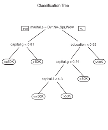
Visualization
If you use the statement below, you can write a new file that will allow you to visualize the tree in Graphviz. The above visualization, however, was done in R and is taken out of the book.
tree.export_graphviz(model, out_file='tree.dot')
Resources I Found Useful:
- Rahul Saxena’s Building Decision Tree Classifiers
- Analytics Vidhya’s Tree-Based Modeling
- Piush Vaish’s Decision Trees in scikit-learn
Mathematicalmonk’s Youtube Explanation (ML 2.1) Classification trees (CART)
This page is a compilation of my notes from the book Data Mining and Predictive Analytics.