A Statistical Analysis of Sentiments
Every four years, the United States goes through the process of electing (or re-electing) its president. Politics becomes a popular topic of conversation, and inadvertently, a popular emotional outlet. Our digital landscape has — mostly textually, but sometimes by video or podcast — granted the ability for people to express their thoughts and feelings on political ideas and events, en masse. Suffice to say, an examination of people’s language in these expressions can yield many useful insights into human (or American) character and the influence of rhetoric on political philosophy and national pride. Therefore, to touch on this examination of language, I will be exploring the sentiments (and their respective confidences), of Tweets pertaining to the first GOP debate, that was hosted on August 6th, 2015.
The Twitter-Sentiment Dataset
The dataset being explored links Tweets to relevant data such as: issues (e.g. abortion), candidates being responded to (and respective confidence), retweet count, and other metadata, but most importantly, sentiments and their respective confidences. We can load our data into an R dataframe with the following code:
Sentiment <- read.csv("~path/Sentiment.csv")
View(Sentiment)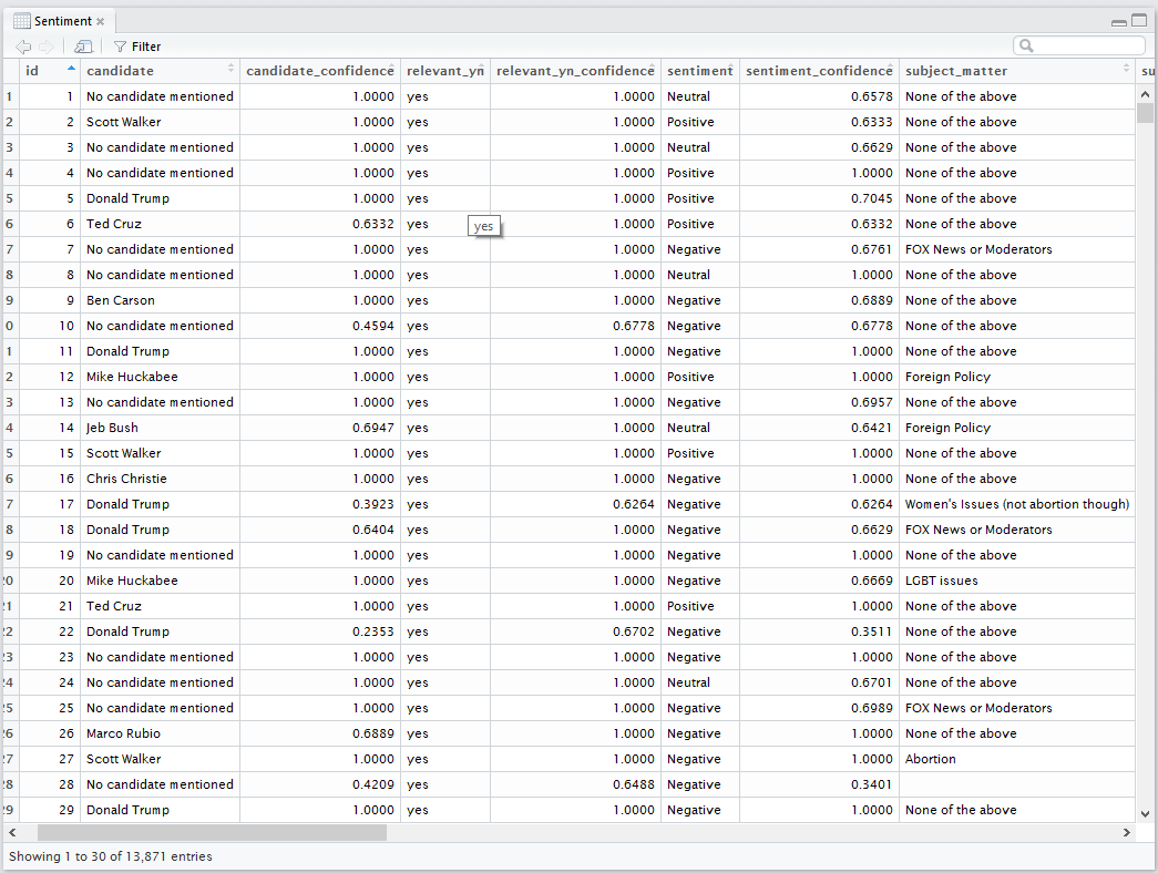
The column labeled sentiment is what we’re interested in so we create two frames, one for negative sentiments, and one for positive. We aren’t worried about neutral.
#Indexes the sentiment confidence for values associated with positive sentiments
(pos <- Sentiment$sentiment_confidence[Sentiment$sentiment == "Positive"])

#Indexes the sentiment confidence for values associated with negative sentiments
(neg <- Sentiment$sentiment_confidence[Sentiment$sentiment == "Negative"])
Confidence Hypotheses
My alternative hypothesis is that the mean confidence of negative sentiments will be greater than the mean confidence of positive sentiments; thus, my null hypothesis is that the mean confidence of negative sentiments will be lower than, or equal to, the mean confidence of positive sentiments. The alternative hypothesis is one-tailed.
Descriptive Statistics of Sentiment Confidences
For this exploration, the mean is chosen as the measure of central tendency because the data is numerical and does not contain outliers. We can find and plot the means of the negative and positive frames quickly.
#Creates a variable for the mean of the indexed positive sentiment confidence levels
(mean_pos = mean(pos))
#[1] 0.7144841

#Creates a variable for the mean of the indexed negative sentiment confidence levels
(mean_neg = mean(neg))
#[1] 0.8003269

#Creates barplot with a y-scale of [0,1]
barplot(c(mean_pos, mean_neg), names.arg = c("Positive Sentiments", "Negative Sentiments"), xlab = "Mean Confidences of Positive and Negative Sentiments", width = .5, xlim = c(0, 2), ylim = c(0, 1), space = .6, col = c("darkolivegreen3", "darkorchid3"), main = "Mean Confidence per Sentiment", ylab = "Mean Confidence Level")

#Creates a dotplot with diamond symbol for better visibility
dotchart(c(mean_neg, mean_pos), labels = c("Negative Sentiments", "Positive Sentiments"), main = "Mean Confidence per Sentiment", xlab = "Mean Confidence Level", color = c("darkorchid3", "darkolivegreen3"), pch = 9)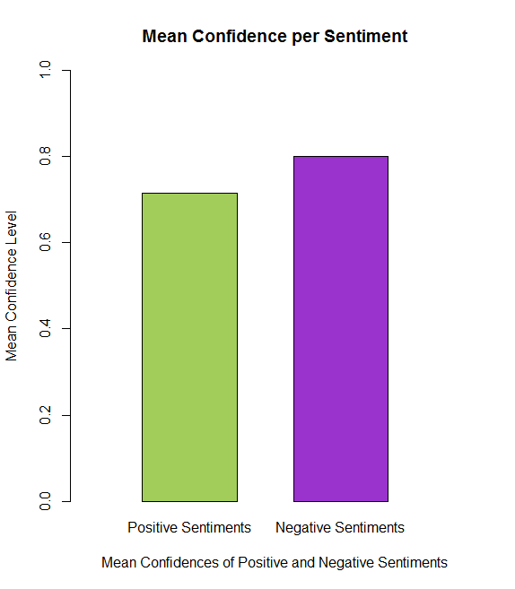
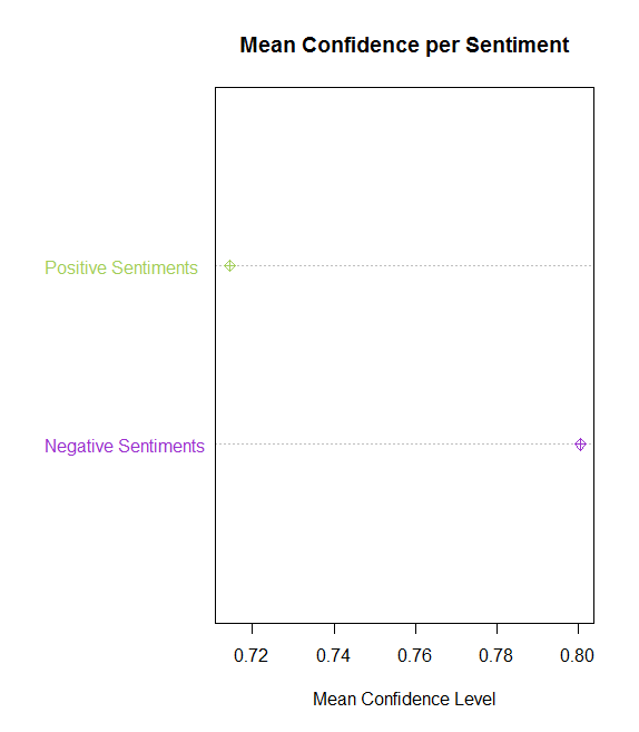
Above, there are two representations comparing the mean confidence levels, per positive and negative sentiment, via the sample provided in the dataset, containing 13,871 observations. The first figure shows the different levels of confidence within the scope of the entire scale (0 to 1). It is evident that the mean confidence for negative sentiments is greater than the mean confidence of positive.
The second figure compares the levels of confidence within the approximate scope of the values themselves (~.70 to ~.81). When calculated, the positive mean confidence is 0.714484 while the negative mean confidence is .800327. Relative to the entire population this is not a large number of observations. Therefore, for a better representation of that population (all Tweets regarding the debate), I will bootstrap resample the observation 10,000 times.
Inferential Statistics
Bootstrapping will also be done with R code:
#Resamples pos vector, takes the mean, then replicates 10,000 times for 10,000 means, stores in variable
(resamples_pos = replicate(10000, mean(sample(pos, replace = T))))

#Resamples neg vector, takes the mean, then replicates 10,000 times for 10,000 means, stores in variable
(resamples_neg = replicate(10000, mean(sample(neg, replace = T))))

#Results in distribution of the difference in negative mean distribution and positive mean distribution, stores in variable
(difference_distro = resamples_neg - resamples_pos)
After bootstrap resampling the data 10,000 times, the calculated means are: Mean(positive) = 0.714436 and Mean(negative) = .800329, both staying relatively the same, with Mean(negative - positive) = .0859. Further, the difference in these distributions can be visualized.
#Expands margins to fit the entirety of the legend
par(xpd=NA)

#Creates histogram of positive and negative mean distributions for easy comparison
#The add=T argument allows us to add multiple graphs in one plot
positive_distro = hist(resamples_pos, freq = T, col = "darkolivegreen3", xlim = c(.69, .815), ylim = c(0, 1800), main = "Bootstrapped Mean Confidences per Sentiment (10,000 Resamples per)", xlab = "Confidence Level")

#As noted above, add = T adds this histogram distribution to the above histogram
negative_distro = hist(resamples_neg, freq = T, col = "darkorchid3", add = T)

#Creates a legend for the histogram(s) above; inset contributes to position
legend("topright", inset=c(-0.02,0), c("Positive", "Negative"), col = c("darkolivegreen3", "darkorchid3"), lwd = 5)

#Produces vertical lines for the negative sentiment confidence mean, then for positive
abline(v = mean(resamples_neg), lwd = 2)
abline(v = mean(resamples_pos), lwd = 2)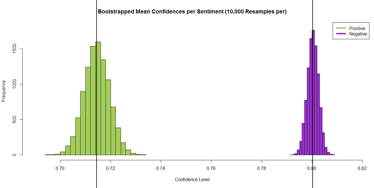
Above, we can see the distributions of resampled means in confidence for both positive and negative sentiments, with the black vertical lines indicating the null hypothesis parameter values. This clearly shows that the mean confidence level is greater for the negative sentiment than it is for the positive. This is useful to visualize, but it might be nice to calculate and plot the actual difference in the distributions.
#Produces distribution of difference between resampled confidences per sentiment
hist(difference_distro, col = "darkslategray3", freq = F, main = "Difference of Mean Confidence Levels between Sentiments", xlab = "Confidence Level", ylab = "Density")

#Defines the C.I. being used for the hypothesis test
#This is also used for the difference distribution
(CI = quantile(difference_distro, c(0.05, 1)))
#        5%       100%
#0.07684648 0.10512917

#Vertical line that shows the C.I. frame
#This is used to determine if null is rejected or not
abline(v = CI, lwd = 2)

#Further verification that neg - pos is not neg or 0, so null is rejected
(mean_diff = mean(resamples_neg) - mean(resamples_pos))
#[1] 0.08579504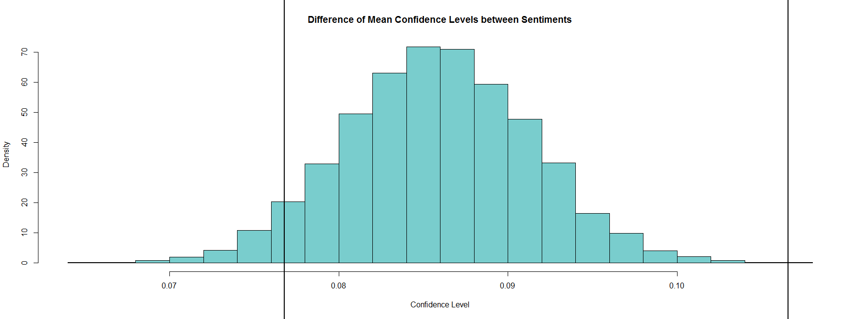
This last figure shows the distributed difference between the mean confidences in negative and positive sentiments. As the hypothesis is being tested with a 95% confidence interval, vertical markers have been placed at the 5% mark (at the value of .0769) and at the 100% mark (at the value of .1103).
Discussion
When assessing the null (neg. mean sent. <= pos. mean sent.), we can conclude that the means are not equal as 0 does not lie within the C.I. frame, and we can conclude that the negative mean confidence is not less than the positive, as there are no negative numbers within the C.I. frame. Therefore, the null hypothesis is rejected and the alternative hypothesis is supported. We can say with 95% confidence that the mean confidence of negative sentiments is greater than the mean confidence of positive sentiments. In other words, in 95 of 100 samples, the difference between the mean confidence of negative tweets and the mean confidence of positive tweets will fall within the given interval.
This might suggest that Twitter could be used, at least in a political context, to vent negative emotions, whether pertinent to politics or not. It could suggest something about these Twitter users in general; perhaps they are mostly liberals, who are more likely to disagree with GOP ideology and be more active online (in social media sites in particular, especially with younger people tending to be more liberal than conservative). Maybe this suggests something about the implicit and explicit nature of positive and negative language, that it’s easier to use and identify negative words than it is to use and identify positive words. Maybe candidates tend to appeal to strong emotions (typically negative) in order to appeal to potential voters. Regardless, there are more variables in this dataset that should be considered. Perhaps responses to Trump, or abortions, greatly skew the sentiments. It may be worth breaking the data down further to account for these variables (presidential candidates and issues). To come to a more significant conclusion, it is necessary to delve further into this data, data like it (other GOP debates, democratic debates, and independent debates), and data relevant to these other considerations.
Disclaimer: A potential issue with this analysis is the algorithm that was used to assess whether a sentiment is neutral, negative, or positive; human intuition can do a much better job in accounting for context, sarcasm, and other subtleties of human language than language-processing algorithms.
Data Source: Kaggle.