Artificial Neural Networks with Sci-kit Learn
The Gist of Neural Nets
A neural network is a supervised classification algorithm. With your help, it kind of teaches itself how to make better classifications.
For a basic neural net, you have three primary components: an input layer, a hidden layer, and an output layer, each consisting of nodes. The nodes of the input layer are basically your input variables; the nodes of the hidden layer are neurons that contain some function that operates on your input data; and there is one output node, which uses a function on the values given by the hidden layer, putting out one final calculation. If this isn’t making much sense yet, don’t worry. It will start coming together.
Each node is connected to every other node in the layers in front of it, so in other words, your input nodes aren’t connected to each other, but they will be connected to every node in the hidden layer, and every node in the hidden layer will be connected to the output node.

The gray lines connecting input nodes to neurons (nodes in the hidden layer) are all weighted. These weights are some value between 0 and 1, and will be multiplied with whatever the input value is. Any node in the hidden layer — let’s say Node_A — will essentially have two functions; a combination function and an activation function. The combination function will likely take the summation of all of the input nodes times their respective weights. Where W is weight and X is input:
**Summation function: **

This is basically saying that for the first node in the hidden layer (which we’ve called NodeA), every connection to it will be summed up. So the first input and its weight is denoted W{1A}X_{1A}. The second input that connects to NodeA and its weight is denoted W{2A}X{2A}, and so forth. The first term W{0A} will always be constant 1, where this term is a constant factor, much like the intercept in regression models.
If we make up some inputs and weights, the equation will look something like this:
$$\text{Net}_A\text{ = (1)(0.5) + (0.4)(0.6) + (0.2)(0.8) + (0.7)(0.6) = 1.32}$$
The resulting 1.32 would then be input into the activation function (likely sigmoid).
**Sigmoid function: **
$$y = \frac{1}{1 + e^{-x}}$$
$$y = \frac{1}{1 + e^{-1.32}} = 0.7892$$
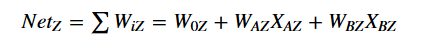
This value is then given to the output node, Node_Z. Node_Z then combines these outputs from Nodes A, B, etc. into a weighted sum (using the weights associated with the connections of these nodes). Now, X_i is treated as the outputs from each node in the hidden layer, and the formula from above is used again.
The sigmoid is used again on the output of $Net_Z$, producing the true output value of the neural network’s first run. Then it’s run again and again for however many data points have been defined.
The weights are what make and break the accuracy of the entire neural network. When the NN is initialized, these weights will be randomized. The neural net then operates and creates its output value, and this value is matched against what it should be. The error is taken, and then the neural net uses some user-defined method to go back through the net to adjust the weights so that the accuracy is maximized, and the error is minimized. If the intuition is still a little cloudy, feel free to take thirty to check the resources at the bottom of the notebook.
import numpy as np
import pandas as pd
import tabulate

from sklearn.preprocessing import LabelEncoder
from sklearn.neural_network import MLPClassifier #you will probably need to update sklearn/conda
from sklearn.model_selection import train_test_split

from IPython.display import display, HTML
pd.set_option('display.notebook_repr_html', True)
df = pd.read_csv("Clem3Training.txt")display(df.head())| age | workclass | demogweight | education | education-num | marital-status | occupation | relationship | race | sex | capital-gain | capital-loss | hours-per-week | native-country | income | |
|---|---|---|---|---|---|---|---|---|---|---|---|---|---|---|---|
| 0 | 39 | State-gov | 77516 | Bachelors | 13 | Never-married | Adm-clerical | Not-in-family | White | Male | 2174 | 0 | 40 | United-States | <=50K. |
| 1 | 50 | Self-emp-not-inc | 83311 | Bachelors | 13 | Married-civ-spouse | Exec-managerial | Husband | White | Male | 0 | 0 | 13 | United-States | <=50K. |
| 2 | 38 | Private | 215646 | HS-grad | 9 | Divorced | Handlers-cleaners | Not-in-family | White | Male | 0 | 0 | 40 | United-States | <=50K. |
| 3 | 53 | Private | 234721 | 11th | 7 | Married-civ-spouse | Handlers-cleaners | Husband | Black | Male | 0 | 0 | 40 | United-States | <=50K. |
| 4 | 28 | Private | 338409 | Bachelors | 13 | Married-civ-spouse | Prof-specialty | Wife | Black | Female | 0 | 0 | 40 | Cuba | <=50K. |
Data Preparation
Overview
Neural networks require numeric inputs. It would be difficult for the algorithm to multiply something like “married” with some weight, and then enter that result into summation and sigmoid functions and get meaningful results. Consequently, every attribute value has to be standardized, taking values between 0 and 1, even for categorical variables. With that said, there is quite a bit to the data preparation stage.
Tidying; Encoding; Balancing
Here, I’m getting a quick feel for the data. How many attributes can we work with? How many unique values are there per attribute? Is there balance between the different potential values? I can also collapse a lot of these specific values into more general ones: “Married-civ-spouse,” “Married-AF-spouse,” and “Married-spouse-absent” can all be collapsed into a ‘y’ representing a married category. The same is done for workclass. Then I print attribute information to answer some of the above questions.
With two unique categories for marital-status, I know I can use the standard LabelEncoder. With 3+ unique categories for workclass and race, I could use OneHotEncoding or create dummy variables. Later I will explain why. Additionally, we can see that there are lower proportions of some races and workclasses. If I wanted a more efficient neural net, I would attempt to balance this so that it can accurately handle these sorts of rare cases. We won’t concern ourselves with that here, though.
#Creates two columns that will be used as their categorical counterparts
df['marital-status-cats'] = df['marital-status'].copy()
df['workclass-cats'] = df['workclass'].copy()

#This dictionary is interpreted as; in column of df, the key will be replaced by the value
category_replacement = {'marital-status-cats' : {'Married-civ-spouse': 'y', 'Married-AF-spouse': 'y', 'Married-spouse-absent': 'y',
                                                'Divorced': 'n', 'Widowed': 'n', 'Separated': 'n', 'Never-married': 'n'},
                        'workclass-cats': {'Federal-gov': 'Gov', 'Local-gov': 'Gov', 'State-gov': 'Gov', 'Self-emp-inc': 'Self',
                                           'Self-emp-not-inc': 'Self'}}
#Reduces the number of categories
df.replace(category_replacement, inplace=True)

print(df['workclass-cats'].unique())
print(df['marital-status-cats'].unique())
print(df['race'].unique())


print(df.race.value_counts())
print(df['marital-status-cats'].value_counts())
print(df['workclass-cats'].value_counts())
print(df['sex'].value_counts())
display(df.head())
['Gov' 'Self' 'Private' '?' 'Without-pay' 'Never-worked']
['n' 'y']
['White' 'Black' 'Asian-Pac-Islander' 'Amer-Indian-Eskimo' 'Other']
White 21391
Black 2379
Asian-Pac-Islander 775
Amer-Indian-Eskimo 241
Other 214
Name: race, dtype: int64
n 13215
y 11785
Name: marital-status-cats, dtype: int64
Private 17385
Gov 3367
Self 2835
? 1399
Without-pay 9
Never-worked 5
Name: workclass-cats, dtype: int64
Male 16709
Female 8291
Name: sex, dtype: int64| age | workclass | demogweight | education | education-num | marital-status | occupation | relationship | race | sex | capital-gain | capital-loss | hours-per-week | native-country | income | marital-status-cats | workclass-cats | |
|---|---|---|---|---|---|---|---|---|---|---|---|---|---|---|---|---|---|
| 0 | 39 | State-gov | 77516 | Bachelors | 13 | Never-married | Adm-clerical | Not-in-family | White | Male | 2174 | 0 | 40 | United-States | <=50K. | n | Gov |
| 1 | 50 | Self-emp-not-inc | 83311 | Bachelors | 13 | Married-civ-spouse | Exec-managerial | Husband | White | Male | 0 | 0 | 13 | United-States | <=50K. | y | Self |
| 2 | 38 | Private | 215646 | HS-grad | 9 | Divorced | Handlers-cleaners | Not-in-family | White | Male | 0 | 0 | 40 | United-States | <=50K. | n | Private |
| 3 | 53 | Private | 234721 | 11th | 7 | Married-civ-spouse | Handlers-cleaners | Husband | Black | Male | 0 | 0 | 40 | United-States | <=50K. | y | Private |
| 4 | 28 | Private | 338409 | Bachelors | 13 | Married-civ-spouse | Prof-specialty | Wife | Black | Female | 0 | 0 | 40 | Cuba | <=50K. | y | Private |
Encoding for Categorical Variables
Above, two different types of encoding were noted: LabelEncoder and OneHotEncoder. Though they both convert categories to numeric values, they behave in different ways. Let’s say I categorize workclass and then use LabelEncoder to create an integer representation of each category. The result will be a 0 for White, 1 for Black, 2 for Asian-Pac-Islander, 3 for Amer-Indian-Eskimo, and 4 for Other. Unless this was ordinal data (like 1st place winner, 2nd, 3rd, 4th), this is unacceptable for the neural network. The neural net would calculate the distance between the first value ‘White’ and the fourth value ‘Other’ and treat this distance as if it’s significant. In our case, each category is equally distant from the other in meaning, and shouldn’t have any superficial scoring like that. So there is an alternative. OneHotEncoder breaks the variable down into a matrix of 0’s and 1’s. If we look at our dataframe, we can match up OneHotEncoder results with the first 16 values of the race column.
t = [[ 0., 0., 0., 0., 1., "White"], [ 0., 0., 0., 0., 1., "White"], [ 0., 0., 0., 0., 1., "White"], [ 0., 0., 1., 0., 0., "Black"], [ 0., 0., 1., 0., 0., "Black"], [ 0., 0., 0., 0., 1., "White"], [ 0., 0., 1., 0., 0., "Black"], [ 0., 0., 0., 0., 1., "White"], [ 0., 0., 0., 0., 1., "White"], [ 0., 0., 0., 0., 1., "White"], [ 0., 0., 1., 0., 0., "Black"], [ 0., 1., 0., 0., 0., "Asian-Pac-Islander"], [ 0., 0., 0., 0., 1., "White"], [ 0., 0., 1., 0., 0., "Black"], [ 0., 1., 0., 0., 0., "Asian-Pac-Islander"], [1., 0., 0., 0., 0., "Amer-Indian-Eskimo"]]
display(HTML(tabulate.tabulate(t, tablefmt='html')))| 0 | 0 | 0 | 0 | 1 | White |
| 0 | 0 | 0 | 0 | 1 | White |
| 0 | 0 | 0 | 0 | 1 | White |
| 0 | 0 | 1 | 0 | 0 | Black |
| 0 | 0 | 1 | 0 | 0 | Black |
| 0 | 0 | 0 | 0 | 1 | White |
| 0 | 0 | 1 | 0 | 0 | Black |
| 0 | 0 | 0 | 0 | 1 | White |
| 0 | 0 | 0 | 0 | 1 | White |
| 0 | 0 | 0 | 0 | 1 | White |
| 0 | 0 | 1 | 0 | 0 | Black |
| 0 | 1 | 0 | 0 | 0 | Asian-Pac-Islander |
| 0 | 0 | 0 | 0 | 1 | White |
| 0 | 0 | 1 | 0 | 0 | Black |
| 0 | 1 | 0 | 0 | 0 | Asian-Pac-Islander |
| 1 | 0 | 0 | 0 | 0 | Amer-Indian-Eskimo |
In essence, each column of numbers represents a possible value of the category (or a possible race). Look at the bottom of the table; there is a record of “Amer-Indian-Eskimo”; note how this is the only occurrence of this race, and there is only one sequence of 10000 in this entire table. The left-most column is reserved for that race, and receives a 1 for any record that has that value for race. Likewise, if you look at the top 3 records, you see the code 00001 next to each record of “White.”
Each race basically has a code to itself. Though ‘Other’ is not listed in the first 16 results, we can deduce that its code is 00010. These values follow neural net input requirements and will be accepted. In relation to each other, the variables are treated fairly and equidistantly. Pandas has a nice way of creating this for us with the get_dummies method.
#####################################

##CODE BLOCK FOR VARIABLE ENCODINGS##

#####################################

#Encoding Income
enc = LabelEncoder()

#Encoding sex
label_encoder = enc.fit(df['sex'])
integer_classes = label_encoder.transform(label_encoder.classes_)
df['sex-encoded'] = label_encoder.transform(df['sex'])

#Categorizing marital-status, workplacee, and race
df['marital-status-cats'] = pd.Categorical(df['marital-status-cats'])
df['workclass-cats'] = pd.Categorical(df['workclass-cats'])
df['race'] = pd.Categorical(df['race'])
print(df['workclass-cats'].cat.categories)
print(df['marital-status-cats'].cat.categories)
print(df['race'].cat.categories)


dummy_races = pd.get_dummies(df['race'], prefix = 'race')
#display(dummy_races)
dummy_workclasses = pd.get_dummies(df['workclass-cats'], prefix = 'workclass')
#display(dummy_workclass)

df = df.join(dummy_workclasses)
df = df.join(dummy_races)
display(df.head())
Index(['?', 'Gov', 'Never-worked', 'Private', 'Self', 'Without-pay'], dtype='object')
Index(['n', 'y'], dtype='object')
Index(['Amer-Indian-Eskimo', 'Asian-Pac-Islander', 'Black', 'Other', 'White'], dtype='object')| age | workclass | demogweight | education | education-num | marital-status | occupation | relationship | race | sex | ... | workclass_Gov | workclass_Never-worked | workclass_Private | workclass_Self | workclass_Without-pay | race_Amer-Indian-Eskimo | race_Asian-Pac-Islander | race_Black | race_Other | race_White | |
|---|---|---|---|---|---|---|---|---|---|---|---|---|---|---|---|---|---|---|---|---|---|
| 0 | 39 | State-gov | 77516 | Bachelors | 13 | Never-married | Adm-clerical | Not-in-family | White | Male | ... | 1 | 0 | 0 | 0 | 0 | 0 | 0 | 0 | 0 | 1 |
| 1 | 50 | Self-emp-not-inc | 83311 | Bachelors | 13 | Married-civ-spouse | Exec-managerial | Husband | White | Male | ... | 0 | 0 | 0 | 1 | 0 | 0 | 0 | 0 | 0 | 1 |
| 2 | 38 | Private | 215646 | HS-grad | 9 | Divorced | Handlers-cleaners | Not-in-family | White | Male | ... | 0 | 0 | 1 | 0 | 0 | 0 | 0 | 0 | 0 | 1 |
| 3 | 53 | Private | 234721 | 11th | 7 | Married-civ-spouse | Handlers-cleaners | Husband | Black | Male | ... | 0 | 0 | 1 | 0 | 0 | 0 | 0 | 1 | 0 | 0 |
| 4 | 28 | Private | 338409 | Bachelors | 13 | Married-civ-spouse | Prof-specialty | Wife | Black | Female | ... | 0 | 0 | 1 | 0 | 0 | 0 | 0 | 1 | 0 | 0 |
5 rows × 29 columns
Looking at the dataframe above, we can see more clearly how both OneHotEncoder and get_dummies work.
Min-Max Standardization for Continuous Variables
Naturally, the numeric data must be standardized as well.
##########################################

##CODE BLOCK FOR MIN-MAX TRANSFORMATIONS##

##########################################

#Standardizing age so numeric values aren't misrepresented in calculations
df['age_mm'] = (df['age'] - (df['age'].min()) / (df['age'].max() - df['age'].min()))

df['education-num_mm'] = (df['education-num'] - (df['education-num'].min()) / (df['education-num'].max() - df['education-num'].min()))
df['capital-gain_mm'] = (df['capital-gain'] - (df['capital-gain'].min()) / (df['capital-gain'].max() - df['capital-gain'].min()))
df['capital-loss_mm'] = (df['capital-loss'] - (df['capital-loss'].min()) / (df['capital-loss'].max() - df['capital-loss'].min()))
df['hours-per-week_mm'] = (df['hours-per-week'] - (df['hours-per-week'].min()) / (df['hours-per-week'].max() - df['hours-per-week'].min()))display(df.head())| age | workclass | demogweight | education | education-num | marital-status | occupation | relationship | race | sex | ... | race_Amer-Indian-Eskimo | race_Asian-Pac-Islander | race_Black | race_Other | race_White | age_mm | education-num_mm | capital-gain_mm | capital-loss_mm | hours-per-week_mm | |
|---|---|---|---|---|---|---|---|---|---|---|---|---|---|---|---|---|---|---|---|---|---|
| 0 | 39 | State-gov | 77516 | Bachelors | 13 | Never-married | Adm-clerical | Not-in-family | White | Male | ... | 0 | 0 | 0 | 0 | 1 | 38.767123 | 12.933333 | 2174.0 | 0.0 | 39.989796 |
| 1 | 50 | Self-emp-not-inc | 83311 | Bachelors | 13 | Married-civ-spouse | Exec-managerial | Husband | White | Male | ... | 0 | 0 | 0 | 0 | 1 | 49.767123 | 12.933333 | 0.0 | 0.0 | 12.989796 |
| 2 | 38 | Private | 215646 | HS-grad | 9 | Divorced | Handlers-cleaners | Not-in-family | White | Male | ... | 0 | 0 | 0 | 0 | 1 | 37.767123 | 8.933333 | 0.0 | 0.0 | 39.989796 |
| 3 | 53 | Private | 234721 | 11th | 7 | Married-civ-spouse | Handlers-cleaners | Husband | Black | Male | ... | 0 | 0 | 1 | 0 | 0 | 52.767123 | 6.933333 | 0.0 | 0.0 | 39.989796 |
| 4 | 28 | Private | 338409 | Bachelors | 13 | Married-civ-spouse | Prof-specialty | Wife | Black | Female | ... | 0 | 0 | 1 | 0 | 0 | 27.767123 | 12.933333 | 0.0 | 0.0 | 39.989796 |
5 rows × 34 columns
Cleaning the DataFrame
This isn’t really essential, but it would be nice to remove some of the frame’s excess so that it runs faster. Additionally, re-ordering the columns will make it a little bit easier to partition the dataset as well. Putting the target variable at one of the ends, preferably the front, reduces a lot of hassle.
#A little bit of dataframe tidying

#Dropping unnecessary columns
to_drop = ['workclass','race','age', 'hours-per-week', 'capital-loss', 'capital-gain', 'education-num', 'demogweight', 'education', 'relationship', 'native-country', 'marital-status', 'marital-status-cats', 'workclass-cats', 'workclass', 'occupation', 'sex', 'race']
df = df.drop(to_drop, axis = 1)

#Reordering the columns to make it easier to use model_selection function
cols = ['income','sex-encoded', 'capital-gain_mm', 'capital-loss_mm', 'education-num_mm', 'age_mm','hours-per-week_mm', 'workclass_Gov', 'workclass_?', 'workclass_Never-worked', 'workclass_Private', 'workclass_Self', 'workclass_Without-pay', 'race_Amer-Indian-Eskimo', 'race_Asian-Pac-Islander', 'race_Black', 'race_Other', 'race_White']
df = df[cols]
display(df.head())| income | sex-encoded | capital-gain_mm | capital-loss_mm | education-num_mm | age_mm | hours-per-week_mm | workclass_Gov | workclass_? | workclass_Never-worked | workclass_Private | workclass_Self | workclass_Without-pay | race_Amer-Indian-Eskimo | race_Asian-Pac-Islander | race_Black | race_Other | race_White | |
|---|---|---|---|---|---|---|---|---|---|---|---|---|---|---|---|---|---|---|
| 0 | <=50K. | 1 | 2174.0 | 0.0 | 12.933333 | 38.767123 | 39.989796 | 1 | 0 | 0 | 0 | 0 | 0 | 0 | 0 | 0 | 0 | 1 |
| 1 | <=50K. | 1 | 0.0 | 0.0 | 12.933333 | 49.767123 | 12.989796 | 0 | 0 | 0 | 0 | 1 | 0 | 0 | 0 | 0 | 0 | 1 |
| 2 | <=50K. | 1 | 0.0 | 0.0 | 8.933333 | 37.767123 | 39.989796 | 0 | 0 | 0 | 1 | 0 | 0 | 0 | 0 | 0 | 0 | 1 |
| 3 | <=50K. | 1 | 0.0 | 0.0 | 6.933333 | 52.767123 | 39.989796 | 0 | 0 | 0 | 1 | 0 | 0 | 0 | 0 | 1 | 0 | 0 |
| 4 | <=50K. | 0 | 0.0 | 0.0 | 12.933333 | 27.767123 | 39.989796 | 0 | 0 | 0 | 1 | 0 | 0 | 0 | 0 | 1 | 0 | 0 |
Partitioning the Data into Training and Test Sets
df_x = df.iloc[:,1:] #All of the input variables, from sex-encoded onward
df_y = df.iloc[:, 0] #The target variable, income

x_train, x_test, y_train, y_test = train_test_split(df_x, df_y, test_size = .2, random_state = 1)
The data must be partitioned into training and test sets because neural networks are a supervised learning method. You have to feed the model pre-classified data (the training set), and then its classifications are judged on how well they predict the test data. The train_test_split function makes this super convenient.
Building our Neural Net
nn = MLPClassifier(activation = 'logistic', solver = 'sgd', hidden_layer_sizes = (12,), max_iter = 2000, random_state = 3)
%time nn.fit(x_train, y_train)
print("Neural net accuracy: " + str(nn.score(x_test, y_test, sample_weight=None)))
Wall time: 1.56 s
Neural net accuracy: 0.7812Neural Net Parameters
random_stateensures that there is some consistency in sampling every time you run the neural net (which is useful because I’m giving multiple examples here).max_iterbeing set to 2000 ensures that I can run neural nets with many hidden layers, each with many neurons, otherwise my examples below might raise an iteration error.Logistic
activationis saying that the NN uses a sigmoid activation function.solverdetermines how the algorithm is going to go through the neural net to adjust the weights (for the sake of minimizing error and increasing accuracy), and for this exercise I’ve used ‘sgd’ or ‘stochastic gradient descent’ because it’s a quicker method than the standard gradient descent. The standard descent goes through every data item, while its stochastic counterpart uses a random sample. Stochastic back-propagation also attempts to guard against getting stuck in any local minima (the algorithm is searching for the global minimum, the smallest amount of error possible). In other words, looking at an error curve, as weights are adjusted the error curve will peak, dip, and bend, and there will likely be multiple dips, but the algorithm is searching for the deepest dip, and not any of the other shallow dips.hidden_layer_sizesis a beast deserving of its own section.Number of hidden layers: Looking at hidden_layer_size in the table below, you may see one number, e.g. the first column is (5, ). Some of the values hold two numbers (5, 5), or more. If you see one number, that means there is one hidden layer. So (5, ) represents a single hidden layer, while (5, 5) represents two hidden layers, and so forth.
Number of neurons in the hidden layer: The actual number that you’re seeing (like 5) is how many neurons sit within that hidden layer. In the table below, in the first column, there are 5 neurons in the hidden layer. In the second column, there are 5 neurons in the first hidden layer, and 5 neurons in the second hidden layer. Go to the last column, there are 100 neurons in the first hidden layer, 100 in the second hidden layer, and 100 in the third hidden layer. Though I’ve used consistent numbers throughout each hidden layer, you could just as well have variations, like (15, 10).
table = [["hidden_layer_size", "(5, )", "(5, 5)", "(15, 15)", "(20, 20)", "(100, 100)", "(20, 20, 20, 20)", "(60, 60, 60, 60)", "(100, 100, 100)"],
         ["Processing time", "337 ms", "4.61 s", "3.27 s", "1.88 s", "25.9 s", "523 ms", "705 ms", "2.13 s"],
         ["Accuracy of neural net", 0.7714, 0.7714, 0.7820, 0.7714, 0.7900, 0.7714, 0.7714, 0.7714]]

display(HTML(tabulate.tabulate(table, tablefmt='html')))| hidden_layer_size | (5, ) | (5, 5) | (15, 15) | (20, 20) | (100, 100) | (20, 20, 20, 20) | (60, 60, 60, 60) | (100, 100, 100) |
| Processing time | 337 ms | 4.61 s | 3.27 s | 1.88 s | 25.9 s | 523 ms | 705 ms | 2.13 s |
| Accuracy of neural net | 0.7714 | 0.7714 | 0.782 | 0.7714 | 0.79 | 0.7714 | 0.7714 | 0.7714 |
An Optimal Number of Layers and Nodes
Looking to the table above, you see some peculiarities:
- (15, 15) takes longer to compute than (20, 20, 20, 20) and even (100, 100, 100)
- Accuracy dramatically drops when going from (100, 100) to (100, 100, 100)
There are more, but the second interestingly points us to some important rules when determining the number of layers and nodes to use in the model. Increasing the number of hidden layers beyond 2 is arbitrary and decreases the power of back propagation (the algorithm that helps neural networks shine, by going backwards and altering input weights for increased accuracy). As for speed, I’m not quite sure why that happens, but a guess would be that when you have more hidden layers, the libraries do better in utilizing more CPU cores than less. If you use other libraries like Tensorflow, you can opt to use the GPU to run the network instead.
jj_ from StackExchange shares Jeff Heaton’s criteria for choosing how many neurons to use:
How many hidden nodes/neurons should I use?
The number of hidden neurons should be between the size of the input layer and the size of the output layer.
The number of hidden neurons should be 2⁄3 the size of the input layer, plus the size of the output layer.
The number of hidden neurons should be less than twice the size of the input layer.
We can calculate this optimal number of neurons easily—visually, even, by looking at our dataframe header and counting the input variables. From ‘sex-encoded’ to ‘race_White’, we have 17 input nodes. Neural nets always have one output node. Using the second criterion, (17) * (2 / 3) + 1 = 12. All of the listed criteria are fulfilled; 12 is less than twice the size of the input layer (34) and is between the size of the input layer and the size of the output layer (between 1 and 17).
Shown above, using one hidden layer and 7 neurons in that layer, we get an accuracy of 0.7812. It might be tempting to hack at the neural net to try to get a higher accuracy, but you would be lying to yourself. It isn’t healthy to have the neural net learn the training dataset too completely, because then you have a neural net that is really close to the heart of your dataset, but can’t be generalized to new data. This is known as overfitting. That isn’t to say that it is not worth putting in a great effort for squeezing out any little bit of legitimate accuracy that you can. For products that scale, even a tiny amount of accuracy can do a lot of good or harm.
Resources:
Sklearn Documentation MLPClassifier is one of Sklearn’s neural network models, in which MLP stands for multi-layer perceptron.
Understanding Neural Networks with Tensorflow Playground This is an awesome resource for gaining an intuition about how neural nets work. You can play with their model, adding and subtracting hidden layers and neurons, to see how the data’s dimensions are reduced, and how its values are transformed in space. Visualizing what the sigmoid function is actually doing is super helpful.
Visualizing Representations This set of visualizations is linked in the previous resource but in case anyone glosses over it, it’s also helpful in that there are real-world examples regarding language and textual data.
This page is a compilation of my notes from the book Data Mining and Predictive Analytics.