Path-Distance Analysis

//This is a fictitious scenario//

Let’s suppose we’re a team of highly skilled NGA agents. We just received a briefing about some suspicious activity between two rival factions. These factions are typically hostile towards each other, but a trusted informant has brought forward some intel suggesting the two factions have been cooperating.

Our team must assist in verifying these claims. Wielding the all-powerful eye in the sky — or, an array of US Government satellites — we will first identify which outposts are linked to each faction, and we will then infer the inter- and intra-faction transportation networks. This will prove valuable to our client, giving them direction when choosing what to surveil so that they can confirm or deny the informant’s claims — that these two factions are indeed working together.

The two factions are indicated by stars and all of the outposts are indicated with green points.

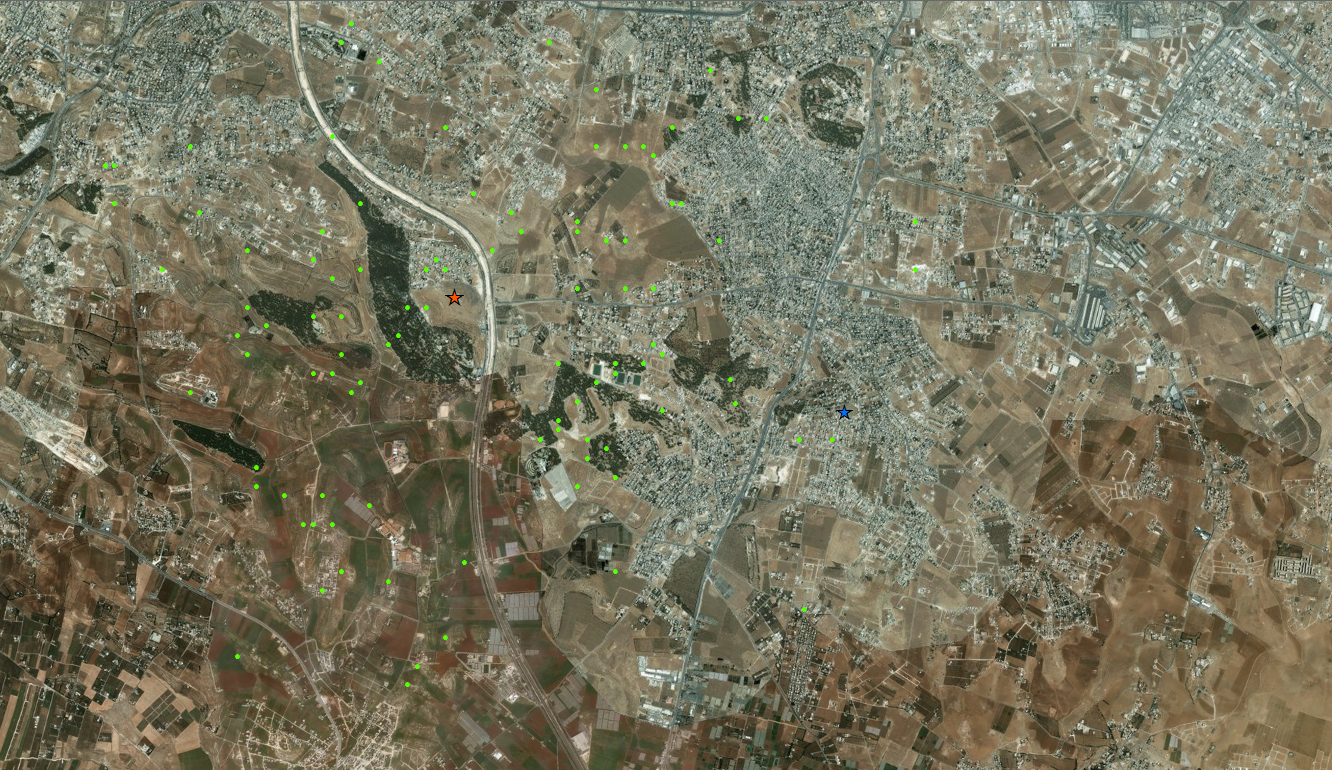
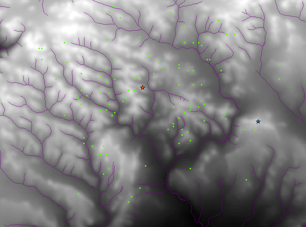
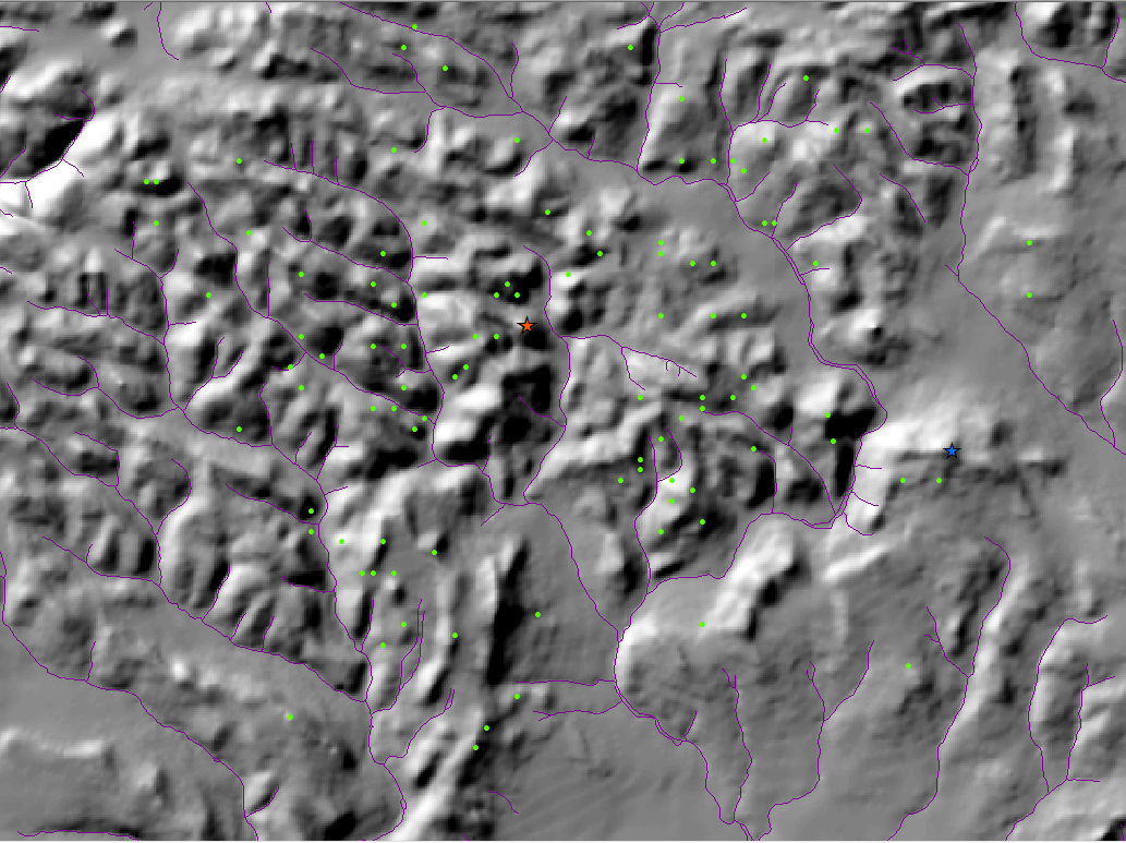
So we have this overview. By itself, it isn’t all that helpful. We need more data if we want to find out which factions own which outposts. Naturally, being the National Geospatial-Intelligence Agency, our team has some useful road-quality data associated with the area.

Methods in Path-Distance Analysis

The objective is to find out which green points are associated with which stars. You can think of each star as a sort of command post. If we think about it, it’s most likely a matter of proximity. You don’t want your outposts in enemy territory. So we want to look at path-distance. But it isn’t so black and white.

Euclid’s Distance

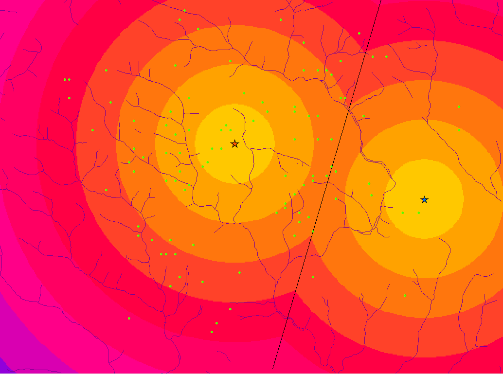
Euclidean distance is basically straight-line distance. Below, you can suppose that each ring is approximately a mile long.

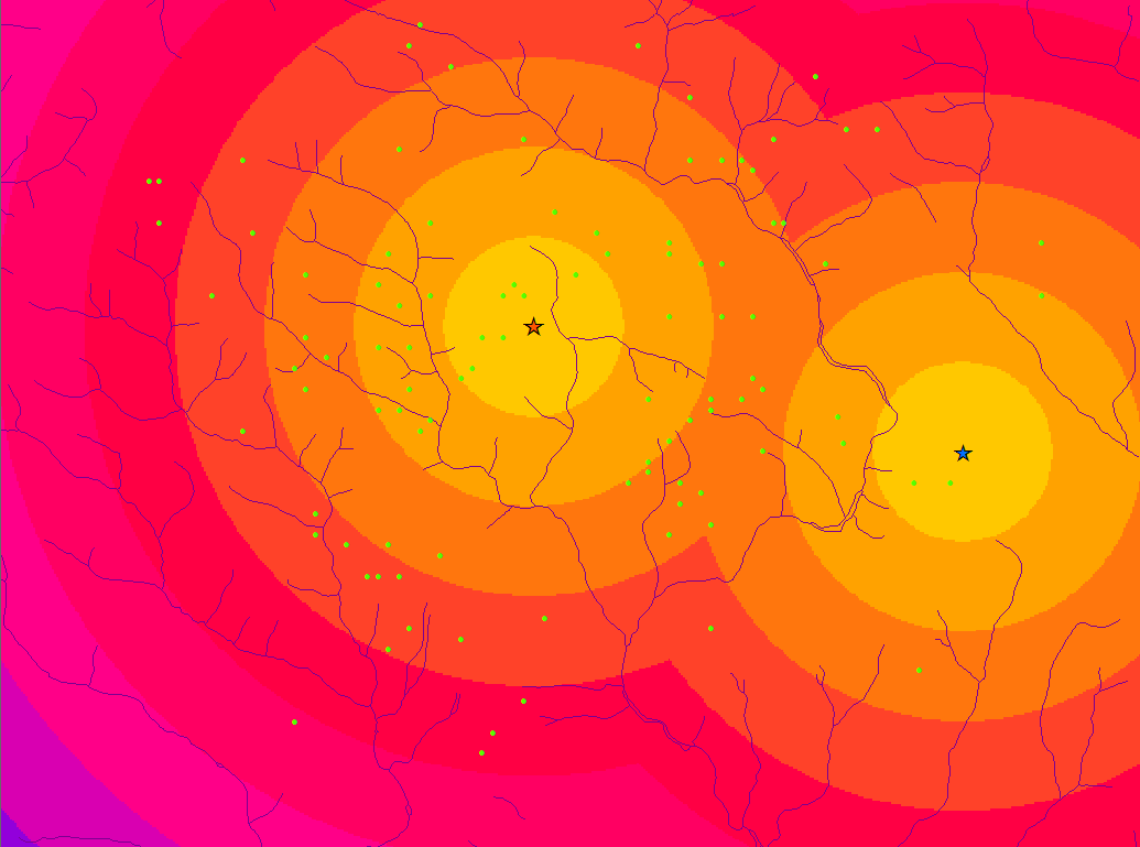
And if this method were right, we could just find where the rings intersect, divide the area into two, and observe where the outposts fall. If the outposts are in the half containing the red faction, the red faction owns them. If the outposts are in the half containing the blue faction, the blue faction owns them.

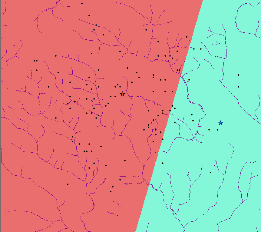
Unfortunately, paths are more complex. Terrain, wind, road condition, stop-lights, and other elements can influence time to get from point A to point B; you simply can’t walk through a mountain. Lucky for us, there are other means of calculating the true distance of paths.

ArcGIS Path Distance

ArcGIS doesn’t suffer the pitfalls of the Euclidean method when calculating distance; it comes equipped with a very versatile Path Distance function. As noted, certain environmental factors can slow you down or speed you up on a given path. The ArcGIS function can account for these factors.

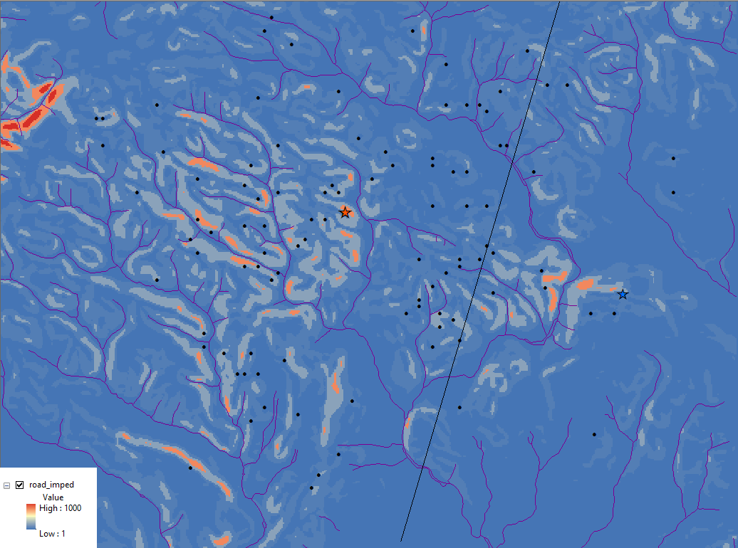
The Path Distance function requires a cost surface, so we will build one. This cost surface is a raster that shows the level of effort required to traverse some area. For simplicity, we will use road quality to account for cost, but GIS software can do a ton more, mathematically incorporating a huge variety of other factors. Intuitively, red areas indicate awful, destroyed roads.

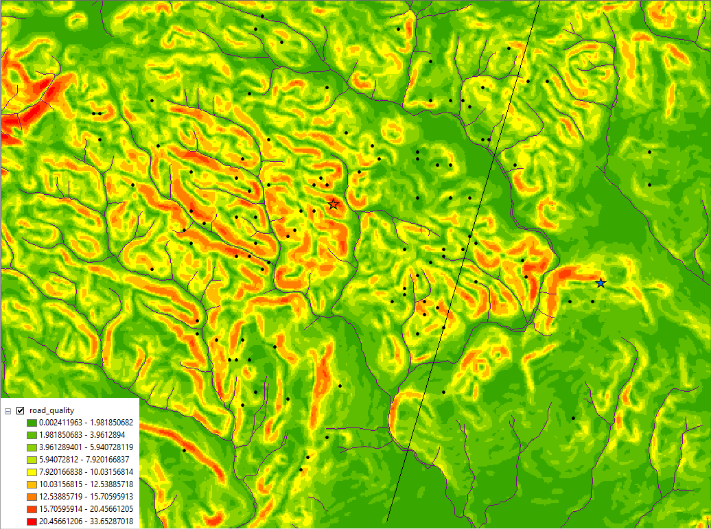
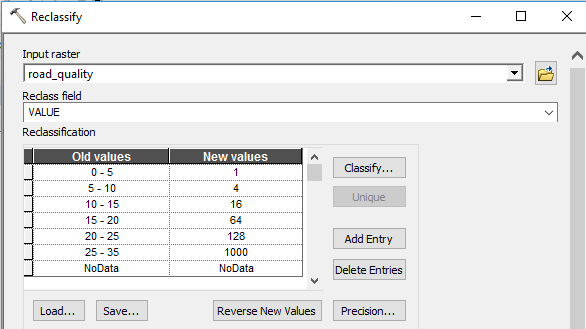
We can then reclassify these data. Values are reclassified to more accurately portray cost. In this case, values rise exponentially to reflect how much more effort is used to traverse the different roads. Using a road under full construction isn’t possible. Reclassifying data accounts for the relativity of the situation at-hand, as driving a car down a bumpy road will have a different cost than walking down the bumpy road.

Path Distance and Backlink Rasters

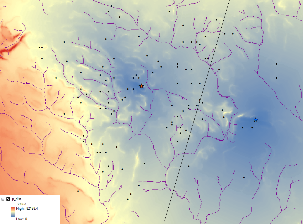
Now we can use our Path Distance function. It uses our command posts (the stars) as input points and it uses our cost raster and surface raster to calculate the cost of navigating the area. It will create two new rasters. One is the path distance model and the other is the backlink raster.

Path Distance Raster

Every cell in this raster holds the least cost accumulated. To put this more simply, it says that we’re starting at a command post (either, it doesn’t matter which). But we want to leave, without having defined any place we’re going. So we start walking. Each step we take, we will have a number of directions we can go, some with higher cost than others (because of road-quality changes). If we think about this in terms of cells, we’re on some given cell, and the cells around it have associated cost values. This new raster shows the least cost path whichever way you want to go.

Backlink Raster

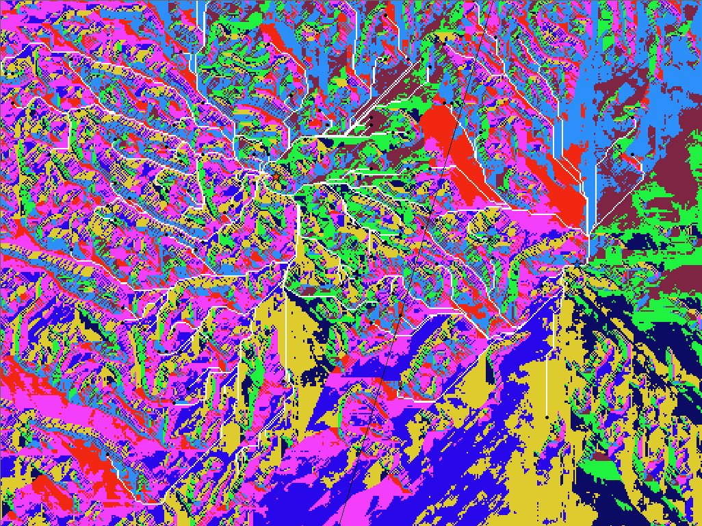
The backlink raster is basically a way-finder, from any (and every) cell, back to the origin (our command posts). The graphic may be a complete mess, seeming entirely incoherent. It’s actually really cool though. Each color is associated with a number, and each number is associated with a direction.

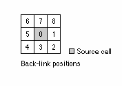
The number 7 tells you to go north, which in our case is the color yellow. And you follow its directions because it is the least-cost path. In other words, your cell is yellow and telling you to go north because the other cells (NE, E, SE, S, SW, W, NW) all come at a higher cost. Think of it as a color-coded way of getting out of danger.

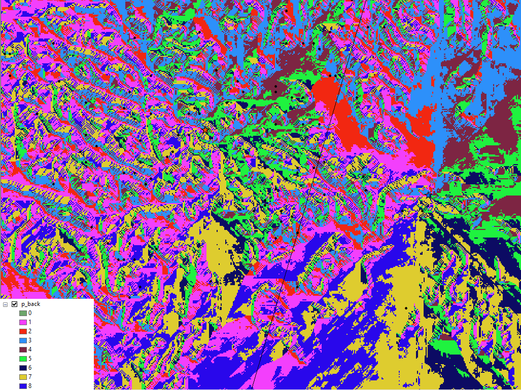
The backlink raster will be used to calculate the true relationship between the two command posts and the dozens of outposts. The Cost Path tool takes the smaller outposts as starting points, then uses the instructions of the backlink to make their way back to the command posts.

…Or to make it a little more clear:

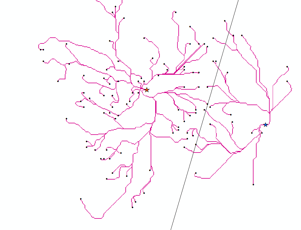
Awesome. So we can finally see the relationships. In this case, it just so happens that Euclid’s method was pretty close, it just missed almost all of the points that were immediately on the other side of the division line. Though it took a little extra calculation, factoring in other variables like road-quality turned out to be worth it.

Inferring Transportation Routes with Corridor Analysis

Corridor analysis finds the optimal corridor between two points. This is essentially finding the optimal areas of transportation, as opposed to one explicit path. The Corridor tool requires two path distance rasters. Each raster will have least cost paths surrounding some source, in our case, a command post.

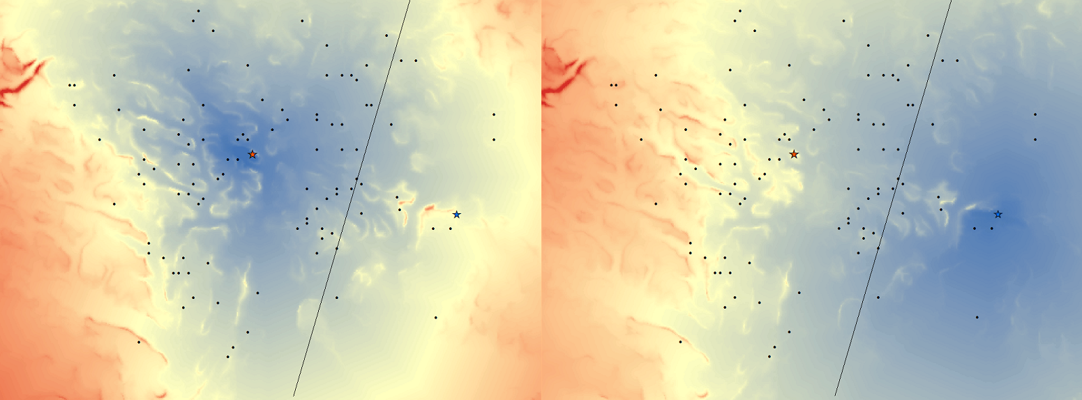
The two rasters will then be summed:

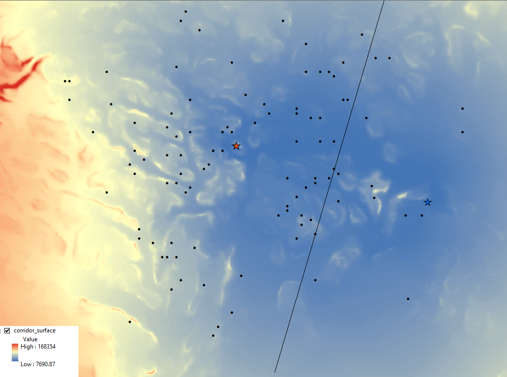
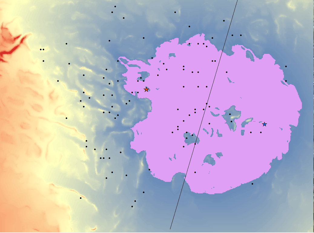
This corridor is hardly insightful. There is too much area between the two factions where transportation is low-cost. We can create thresholds to check for smaller values, so that we can narrow down the number of potential routes. This is done with conditional statements. We’re trying to highlight lower-value areas and according to the key, the range of data is [7,690-168,354]. These data vary between projects so trial-and-error is really the best bet for finding a threshold we like. Using Raster Calculator, we will first try finding data that is less than 10,000 with our conditional statement.

Con(“corridor_surface”<10000,1) — For each cell, if cell value is less than 10,000, write 1 to cell in output raster.

Con(“corridor_surface”<9000,1) — For each cell, if cell value is less than 9,000, write 1 to cell in output raster.

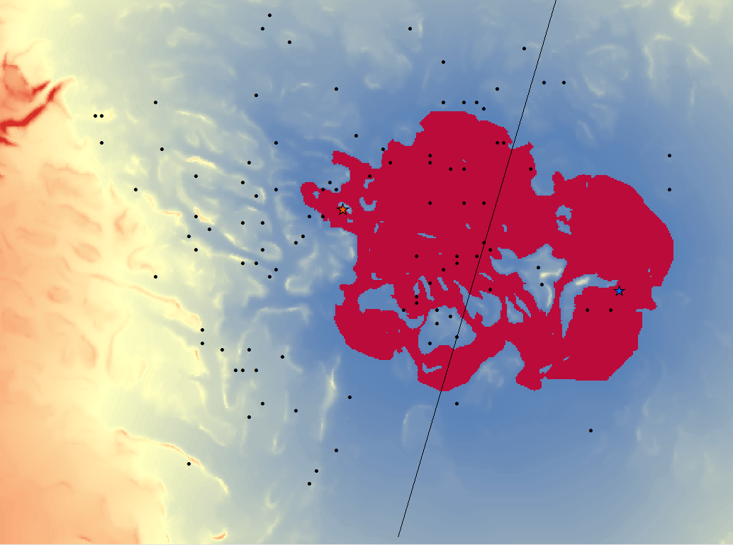
Pretty good, but we can narrow it down just a little more.

Con(“corridor_surface”<8400,1) — For each cell, if cell value is less than 8,400, write 1 to cell in output raster.

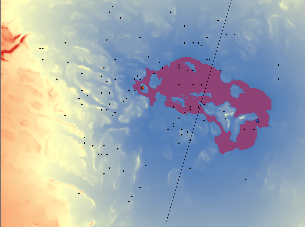
This is good enough. If we narrow it down too far, we would be unreasonably assuming that these factions use the most optimal route possible to travel between command posts. This isn’t realistic. Fortunately, this threshold served its purpose in narrowing down possible routes enough to be insightful. There are three major bottlenecks that could be strategically used to switch out vehicles when tailing a target.

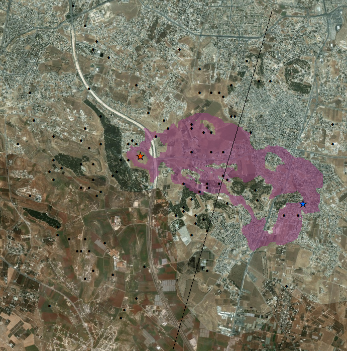
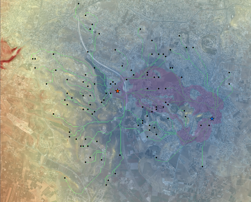
With our GIS, we have now inferred the relationship between the two factions and the marked outposts. We also created a great deal of actionable intelligence regarding factions’ transportation networks. From this, we can consider which areas might be at-risk to violence; which outposts are weaker due to having a low degree of centrality within its faction’s network; which outposts are likely to be hotspots; and which areas a surveillence team might work most effectively in.

Data Source:

The University of Arizona

Advanced GIS (GIST 420)

Professor Gary Christopherson

The data used comes from class exercises not related to this scenario.