My Introduction to GIS with Python

Python is a powerful tool in the GIS world, so I wanted to get a little bit of practice with it. I have had a lot of fun working with the Global Terrorism Database so I figured I would go from its CSV format to one that is better-supported by GIS — the shapefile. The dataset contains information related to terrorist attacks, including attack locations. Each location has a variety of data but I will focus on country, latitude, and longitude. Specifically, I will observe attacks in Iraq. The coordinates are based on WGS1984 standards, so they will have to be converted to UTM Zone 38N in order to be mapped on a flat-surface (more on this later, no worries if you don’t understand).

First Step: Cleaning the Data

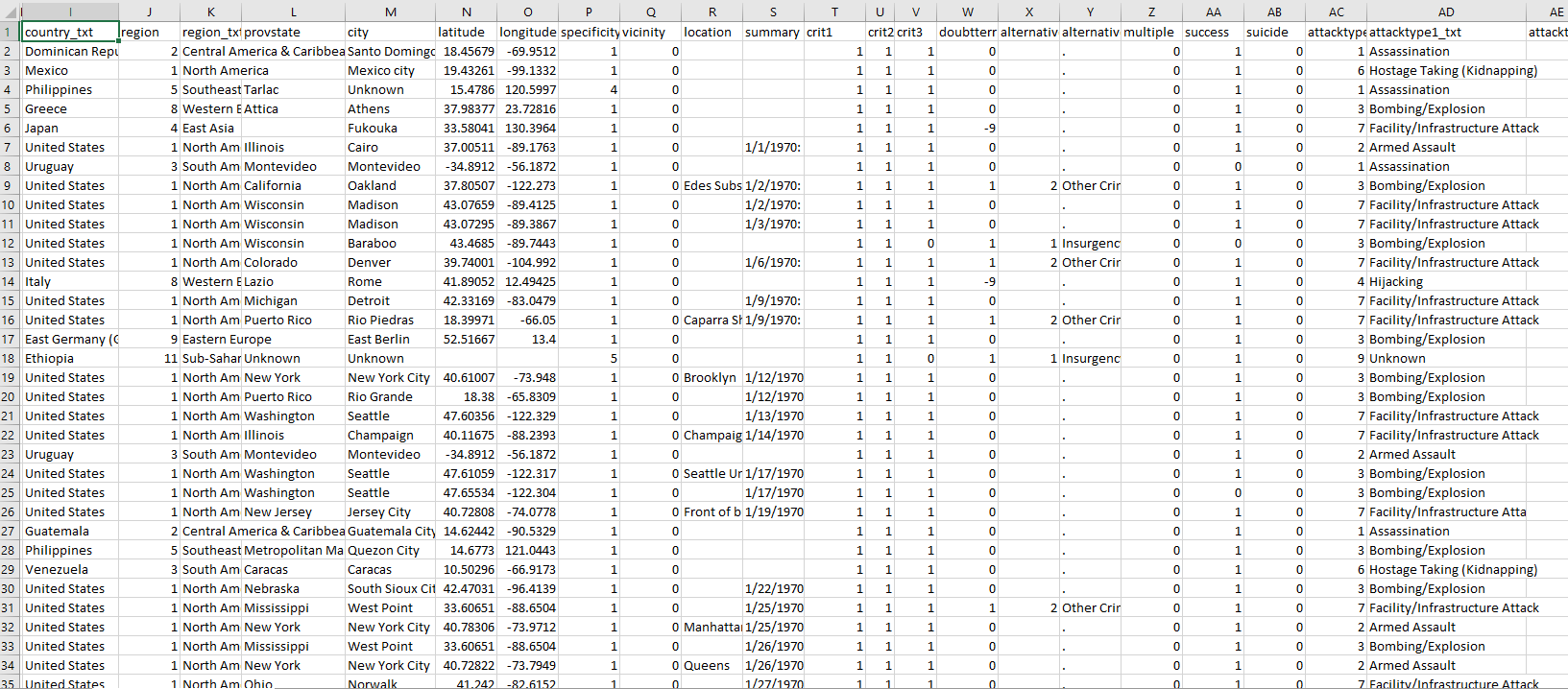
When we first get the data, it contains way more information than we need. There are over 120 variables and as noted, we primarily want to focus on locational data and a few other variables like target type, attack type, and terrorist group responsible. We need to get rid of excess so that our script runs faster and is more relevant to our objective.

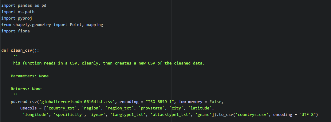
You can see the list of imported modules. Pandas is used first to load the data into a DataFrame (basically a table) to be operated on. Functional programming is best suited for the overall task, as for most data analysis, so here is a simple function to clean the data:

In the event that the clean_csv() hasn’t been called yet, call it. If it has already been called, don’t worry about it.

Now we’ve cleaned our data and created a DataFrame with most of what we want. Now we can use another function to specify which country we’re interested in.

Second Step: Specifying the Country of Interest

In our case, we’re interested in looking at Iraq. We want to see all of the terrorist attacks that occurred in Iraq. We will clean the frame a little bit more now. This step could have been done in the first function but I believe it’s more simple for a future user to read, understand, and plug the country of interest with a separate function.

Simple enough. The DataFrame object from the last function is loaded in and we create a new frame that meets our criteria; where every record’s country value is “Iraq.” Then, any records containing NaNs are dropped. Our coordinate data is still based on the WGS1984 standard — they work on 3D planes, like in Google Earth, but not on 2D planes, like almost every other map in existence. This calls for conversion.

Third Step: Converting the Coordinates

Coordinate systems use values that assume 3D-space and are provided by satellites. The problem is, most maps are flat, and when you’re flattening the earth there are always distortions. These distortions affect distance, direction, and scale. Check out Kai Chang’s awesome visualizations for comparing different map projections.

Mathematical formulae are used to convert geographic coordinates into their flat-plane equivalents. The Python module Pyproj handles this for users, so I import this module and use it in my conversion function.

You may have noticed I used the UTM projection (Universal Transverse Mercator). This is because distortion occurs at the poles of the earth, whereas the areas around the equator tend to be accurately preserved. This is good for us since we’re observing Iraq. Iraq falls in the Zone 38N band, and must be used as an argument.

Incorrect Pyproj Value Output

Here, I made a common mistake. I was getting pretty wildly wrong values, where points were showing up in Ethiopia and not Iraq. Note the values for utm_lat and utm_lon toward the bottom:

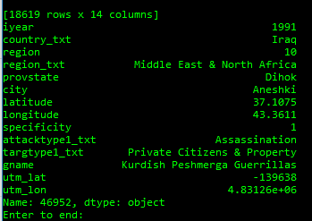
I wanted to verify whether or not these values were right, because I knew upon plotting them, I was getting Ethiopian areas, so I used the Geographic/UTM Coordinate Converter Website.

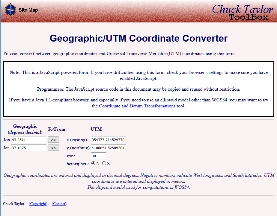
Upon looking at the UTM outputs, this is obviously wrong:

• -139638 != 354377
• 483126 != 410805

My problem was that I had the parameters switched. In simple terms, I had p2(latitude, longitude), but I should have had p2(longitude, latitude). It turns out, in many Python GIS modules, longitude comes before latitude. When I changed the order of these parameters, the output was correct.

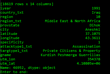
Now that all of the outputs are correct, we can go to the final step.

Fourth and Final Step: Producing a Shapefile with our New Data

To create a shapefile I decided I would use Python’s Fiona and Shapely modules.

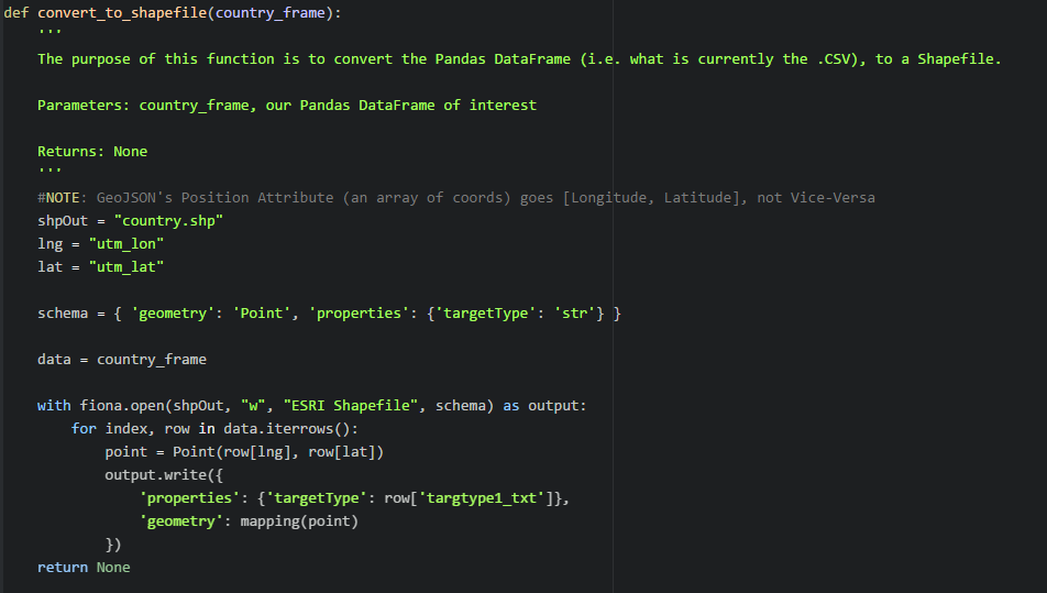
The previous two functions are called:

Now the shapefile has been created:

Using ArcGIS to Map the Shapefile

Open ArcMap. Go to the Catalog tab and click it. Navigate to the folder. Find the shapefile.

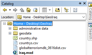
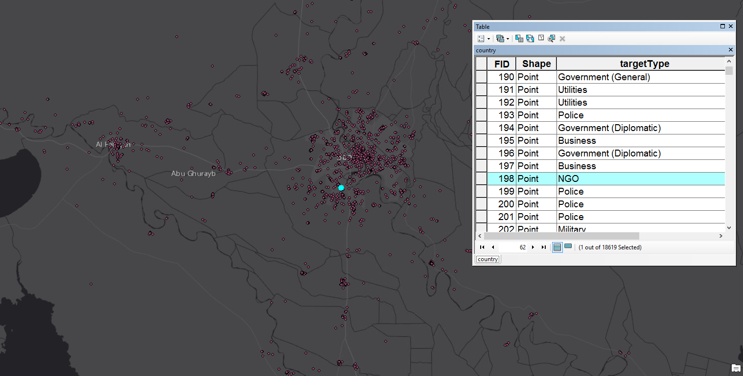
Right click the shapefile. Go to properties. In the ‘XY Coordinate System’ tab, expand the ‘Projected Coordinate Systems’ folder, expand UTM, expand WGS 1984, expand Northern Hemisphere, and then find ‘WGS 1984 UTM Zone 38N.’ Click it and press the ‘Apply’ and ‘OK’ buttons. Drag the shapefile onto your canvas. And don’t forget to go to ‘Add Data’ and ‘Add Basemap’ to find a map to sit under the points — I chose the dark gray basemap.

As the code indicated, I was also recording information on the target types of the attacks. When I use the identify tool on a point (or attack location), or when I open the attribute table, this information will be associated with the geometry (in our case, the point).

Conclusion

These functions are simple but they have vast implications. All I did was take a CSV with spatial data, filtered out data that I wasn’t interested in, transformed the data into something that I could actually work with, and then wrote the data to a shapefile. These processes give me the ability to do further geospatial analysis and to build and deploy an interactive and informative website regarding terrorist attacks. In the future, I definitely intend to take advantage of other Python geospatial libraries for map-making, like Descartes and Basemap.